Writing a panel-method solver in Zig

I’ve been flying soft wings for years without really understanding the sections they’re built from. Paragliders, speedwings, kites — they all live or die on the shape of a slice through the wing, and I’ve mostly taken that shape on trust. So I’ve started building something to fix that: a simulation backend called Camber, which takes a wing section, an angle, and an airspeed, and tells you what the air does about it.

This is the first of what I expect to be quite a few posts. It covers the part that works: the panel method. My maths is not strong, so I’ve had to build the intuition first and let the equations follow, and that’s how I’m going to explain it. If you can picture air moving, you can follow all of this.

Two stories about air

Air behaves in two completely different ways depending on how close to the wing you are, and almost every practical aerodynamics tool is built on that split.

Nearly everywhere, air is so slippery that friction may as well not exist. It just has to flow around the shape rather than through it. Solve that, and you get the pressure everywhere on the surface — and pressure is where lift comes from.

Then there’s a film glued to the surface, about one percent of the chord thick, where friction is the only thing that matters. That film is where drag comes from, and where stall comes from.

This post is entirely about the first story. It’s the easier one, it runs in about a millisecond, and it gets you lift and pressure. The second one is much harder, I’m still fighting it, and it’ll get its own post.

A wing is a list of points

The first job is turning “NACA 4412” into something a computer can chew on. You walk all the way around the section and write down coordinates, then join consecutive points with straight lines. Those straight segments are the panels.

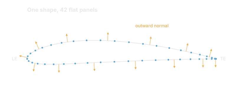
Two details in that picture do real work.

The points aren’t evenly spaced. They’re bunched at the nose and the tail using a cosine distribution. Over the middle of a section the flow does almost nothing interesting — the pressure changes gently and slowly. Around the nose it goes berserk: air comes to a dead stop, then accelerates to well above freestream speed within a couple of percent of chord. Even spacing would spend most of your panels describing the boring part and smear the most important feature on the whole surface.

And the direction you walk matters. I go clockwise — tail, along the bottom, round the nose, back along the top. Every panel computes its outward normal as “the direction I’m travelling, rotated ninety degrees”. Walk the other way and every normal points into the wing, and the sign of the lift flips. I have this written in capital letters in my notes.

The trick: throw the wing away

Here’s where it gets clever, and where I had to stop and think for a while.

You’d assume you solve the flow around a solid object. You don’t. You delete the object entirely and replace its surface with a vortex sheet — imagine laying a carpet of tiny spinning rollers along where the skin used to be. Each roller drags the air around with it.

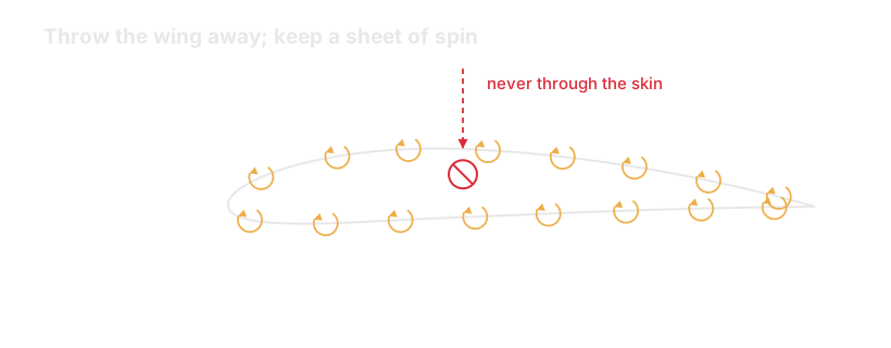
Now ask one question: how hard does each roller have to spin so that the wind plus all the rollers together never pushes air through the line where the skin used to be?

Answer that, and you’ve solved the flow — because a flow that doesn’t cross the skin is indistinguishable from a flow around a solid wing.

Why spinning rollers, specifically? Because spin is what makes lift. You could lay down a carpet of little sprinklers instead, blowing air outwards, and they’d make the shape appear fatter — but they’d generate exactly zero lift no matter how you tuned them. Net circulation around the section is lift. Vorticity is the only ingredient that can produce it.

Chop the surface into N panels, let the spin vary linearly along each one, and the unknowns become the values at the N+1 corners. Then write one equation per panel: at this panel’s midpoint, the flow perpendicular to the surface is zero.

That’s N equations and N+1 unknowns. One short.

The bit where nature has to choose

That missing equation isn’t a bookkeeping mistake. It’s the most interesting thing in the whole method.

Frictionless flow theory genuinely does not have a unique answer. There’s an entire family of valid solutions around any wing section — one for every possible amount of circulation — and every single one satisfies “no air through the skin” perfectly. In one of them the air whips around the sharp trailing edge from below to above. In another it goes the other way. In exactly one, the flow leaves the trailing edge smoothly, both streams merging and departing together.

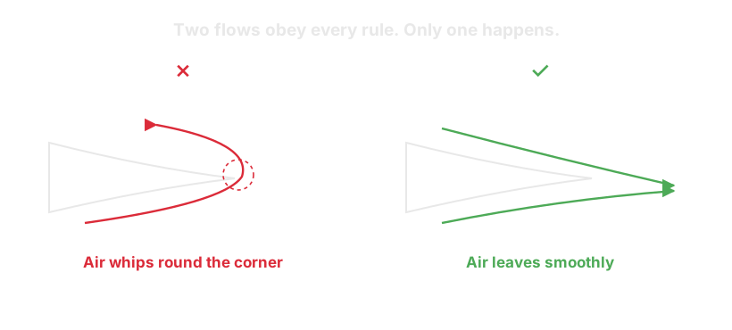
Nature picks the smooth one. It picks it because real air has viscosity, and viscosity flatly refuses to let flow turn a sharp corner at infinite speed. The first attempt to do so sheds a vortex downstream — you can watch this happen in a water tank — and that departing vortex leaves behind precisely the circulation needed to make the trailing edge smooth ever after.

So the missing equation is a fact about sticky air, smuggled into a model that has no friction in it anywhere. In my code it is one line:

// Kutta condition: gamma_0 + gamma_N = 0 (closes the (m x m) system).
a[n * m + 0] = 1.0;
a[n * m + n] = 1.0;

The spin strength just under the tail, plus the spin strength just above it, equals zero. Since the sheet strength turns out to be the local surface speed, that says the speeds on the two sides of the trailing edge match: no jump, no infinite turn.

This is where the lift comes from. Everything else in the file is bookkeeping. When I had a sign error early on and my sections produced negative lift, this was where the bug was.

It’s all one linear system

With that last equation in place you have a square system: a matrix, a vector of unknown spin strengths, and a right-hand side.

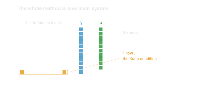
Each entry of the matrix answers a very concrete question: if roller j were spinning at unit strength, how much air would it push through panel i? That’s pure geometry — there’s a closed-form expression involving a logarithm and an arctangent, and it’s the same on every panel method ever written.

The bit worth noticing is what isn’t in the matrix. The angle of attack appears nowhere in it. It only touches the right-hand side. So the expensive half — factorising the matrix, which is the cubic-time part — gets done once per shape, and each new angle is a cheap back-substitution. Running a whole polar sweep across twenty angles costs roughly the same as solving one.

Getting the answer back out

Once you’ve solved for the spin strengths, you might expect to have to sum up every roller’s contribution at every point to find the surface speed. You don’t, and this is my favourite part.

A vortex sheet is defined as a jump in tangential velocity across it. The solution was constructed so the air inside the imaginary body is perfectly still. So the jump across the sheet is simply the speed outside it. The strength you solved for is the speed of the air sliding over the skin.

Then Bernoulli turns speed into pressure — fast air means low pressure — and the whole thing collapses to one line:

const gamma_mid = 0.5 * (gamma[i] + gamma[i + 1]);
cp_arr[i] = .{ .x = geom.xc[i], .cp = 1.0 - gamma_mid * gamma_mid };

Cp is the pressure coefficient: local pressure minus ambient, divided by the pressure you’d get by bringing the freestream to a dead stop. Dividing through like that means it doesn’t depend on how fast you’re going or how thick the air is — the same curve holds at 10 m/s at sea level and 30 m/s at three thousand metres. It’s the universal currency of this field.

Here’s what actually comes out of the binary:

echo '{"naca":"4412","aoa_deg":6,"n_points":200,"re":1000000}' \
  | ./solver/zig-out/bin/camber-solver

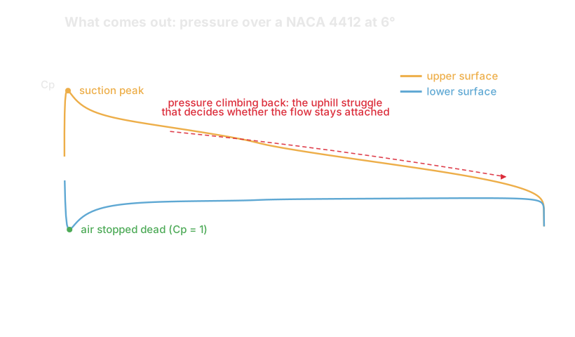
Three things to read off it. Cp = +1, bottom left, is air brought completely to rest — the stagnation point, and the highest value physically possible. The big negative spike just behind the nose is the suction peak, where air is moving far faster than freestream and pressure has dropped well below ambient; most of the lift lives there. And the long climb from the peak back towards zero at the tail is the pressure recovery — air being asked to move into rising pressure. That climb is the whole ballgame for the second story, because it’s what eventually pushes the boundary layer into separating.

The drag that isn’t drag

The solver reports a drag number. It’s a lie, and I’ve had to be quite disciplined about saying so.

In genuinely frictionless flow, a closed body experiences no drag at all. The pressure pushing back on the front is exactly cancelled by pressure pushing forward on the rear. This is d’Alembert’s paradox, and it bothered people for about a century before boundary layers were understood.

So the drag my panel solver computes is not physical. It’s the residue of chopping a smooth curve into flat segments — a measure of how good my panelling is, nothing more. On the run above it’s 0.000172, which is a couple of orders of magnitude smaller than the real drag of that section. If it ever gets large, that tells me my resolution is bad, not that I’ve designed a draggy wing.

I have a rule written into the project: never report this number as drag. It would be very easy to ship something that looks like a working aerodynamics tool and is quietly nonsense.

Two checks that keep me honest

The pressure integration gives lift. But there’s a completely independent route to the same number — Kutta–Joukowski, which says lift is just twice the total circulation. Two different calculations from the same solution:

cl      = 1.2386
cl_circ = 1.2387

If those ever diverge by more than a percent, the solver attaches a warning to its own output. It’s a cheap and brutal test: the two agree only if the solution is actually right.

The second check is that every fast path has a slow twin. The influence matrix is built with SIMD, four panels at a time, and there’s a plain scalar version of the same code that a test requires to agree to floating-point round-off. The optimisation is only safe to keep because the twin exists.

One result that looks like a bug and isn’t: my lift slope comes out at 6.86 per radian, against the textbook thin-aerofoil value of 2π ≈ 6.28. That’s 9.2% high. It’s meant to be. Thin-aerofoil theory linearises the thickness away, and thickness genuinely adds lift. Every thick-section panel method overshoots the textbook line by about this much. It took me an embarrassingly long time to stop trying to “fix” it.

Why Zig

I wrote about first impressions of Zig a while back, and this project has mostly deepened what I liked.

Arena allocators suit this problem perfectly. A solve allocates a lot of scratch — matrices, geometry arrays, per-panel state — and every bit of it dies at the same moment. So you allocate freely from an arena and throw the whole thing away at the end, with no per-object bookkeeping at all.

@Vector(4, f64) gives you SIMD without intrinsics or a library, and it stays readable.

And the discipline that’s paid off most isn’t a language feature but a rule I set early: no global state, everything passed as a parameter. That felt slightly pedantic while writing it. Then I wanted to run six independent validation cases at once, and it turned out there was nothing to synchronise, because there was nothing shared. It just worked, on the first attempt, for a 3.6× speedup.

The thing I still find genuinely hard is the build system. It’s powerful and it’s clean, but 0.16 moved to a module-based build.zig and most of what you’ll find online is written against something older.

What it can’t do

This is worth being blunt about, because a plausible-looking wrong answer is worse than no answer.

There is no viscosity in any of this. So: no real drag, no stall, no separation, no transition from laminar to turbulent flow, no compressibility. You cannot get a glide ratio out of it, because you cannot get drag out of it. You cannot find the stall angle, because nothing in the model knows how to stall — push the angle up and the lift just keeps rising happily, forever, which real wings famously do not.

What it does give you, and gives you fast and accurately, is lift and the pressure distribution for attached flow. That turns out to be exactly the input the second story needs.

Next

The boundary layer. That’s where drag and stall live, and it’s a much nastier problem — the thin film and the outer flow each need the other’s answer, so you end up iterating between two solvers until they stop arguing. I have that working, mostly. I also have a validation gate that it currently fails on two criteria out of five, which I’ll write about honestly, because the failures are more interesting than the passes.

The diagrams in this post were generated from the solver itself rather than drawn by hand, which felt like the right way to do it. If any of it is wrong, I’d genuinely like to know.