The boundary layer, and the test it fails
Back in the spring I wrote about the half of aerodynamics where air has no friction. That half is fast, it is accurate, and it gives you lift and pressure. It also cannot tell you how much drag a wing has, or when it will stop flying — which are, unfortunately, the two things a person choosing a wing actually wants to know.
This post is the other half. It is where drag lives, where stall lives, and where I have spent most of my time since. I have it working, and I have a test written before any of the code that it still fails. The failures turned out to be far more useful than the passes, so most of this is about those.
The film
Everywhere except very close to the skin, air behaves as if friction did not exist. Very close to the skin, friction is the only thing that matters, because air genuinely sticks to solid surfaces. The molecules touching the wing are, on average, going exactly the speed of the wing. A tiny distance away they are going full speed.
Everything friction does to a wing happens in that gap.
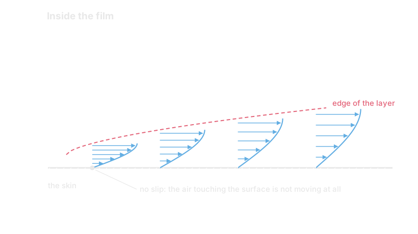
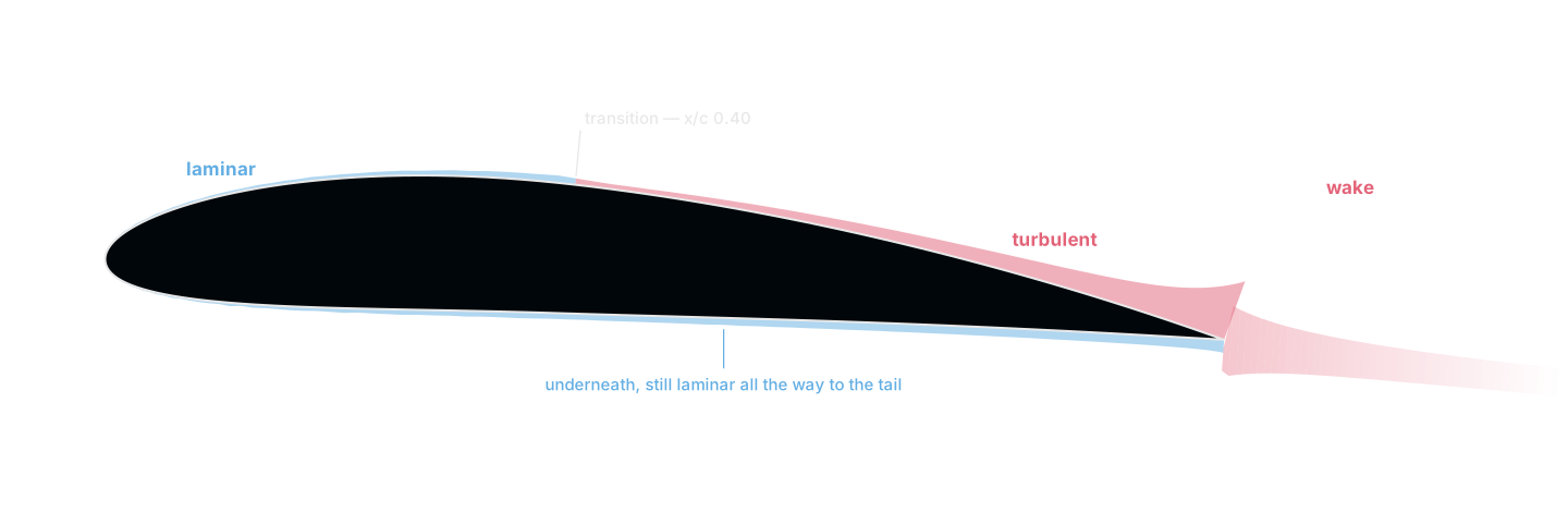
The gap is thin. On the section in the hero image at Re 10⁶ it is about one percent of the chord over most of the wing. That thinness is the entire reason any of this is tractable, because it means the outer flow barely notices the layer exists, and the layer can be solved as if the outer flow were simply handed to it.
Nobody solves the profile
The obvious approach is to work out the actual shape of that velocity curve everywhere, which means solving a partial differential equation over a two-dimensional region for every case. People do this. It is called a Navier-Stokes solve, it takes minutes to hours, and it is not what I want when the point of the project is to sweep a hundred candidate sections.
The trick, and it is a very old one, is to stop caring about the shape of the curve and keep only two numbers per station: how much air is missing, and how much push is missing.
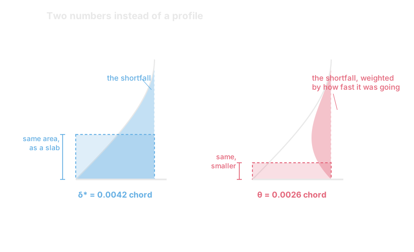
δ*, the displacement thickness, is the first. Add up the air that failed to arrive because of friction, and ask how far out you would have to move the wall to lose that much air from a flow with no friction at all. That distance is δ*. It is the number that matters most here, because it is the only thing about the boundary layer that the outer flow can see: as far as the frictionless solve is concerned, the wing is simply δ* fatter than it really is.
θ, the momentum thickness, is the second. Same idea, but weighting each bit of missing air by how fast it was going. This one is the drag, more or less directly — momentum that the air had at the front and does not have at the back went into the wing.
One number decides everything
Their ratio, H = δ*/θ, turns out to be the interesting one. It says nothing about how thick the layer is and everything about its shape — specifically about how full the profile is near the wall, which is to say how much momentum the flow has left down there to keep pushing itself along.
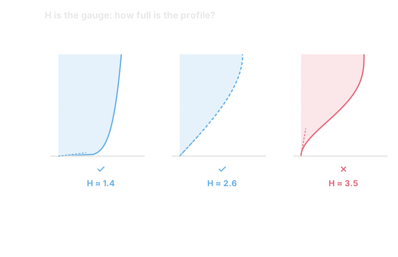
A turbulent layer runs at H ≈ 1.4. It is constantly dragging fast air down from the outside and slinging slow air up, which keeps the wall region energetic — at the cost of far more skin friction. A laminar layer sits around 2.6: much slicker, much less able to cope with anything difficult.
And when the flow is asked to climb into rising pressure — which is exactly what the whole rear half of an aerofoil asks of it — H climbs. Somewhere around 2.4 for a turbulent layer, and nearer 3.5 for a laminar one, the profile runs out of momentum at the wall, the flow stops, and it lifts off the surface. That is separation, and it is the mechanism behind stall.
So the entire drama of a wing section is: how long can you stay laminar (cheap, but fragile), and having gone turbulent (expensive, but tough), can you get to the trailing edge before H runs away?
Waiting for a wobble
The switch between the two is called transition, and it is the single most consequential thing in the whole model, because it decides both the drag and the toughness.
It is not a threshold you cross. A laminar layer is unstable long before it is turbulent: a tiny disturbance at the right frequency grows, exponentially, as it travels downstream. The model I use — the e^N envelope, from Drela and Giles — integrates that growth along the surface and declares the flow turbulent once the most-amplified disturbance has grown by a factor of e^N.
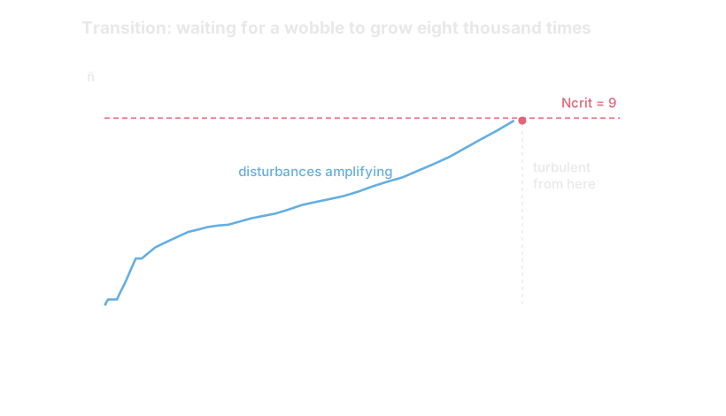
Before this I had Michel’s criterion, which is a local correlation — look up the current state, ask whether it has tripped. It is cheaper and it is consistently wrong here, firing 0.1 to 0.2 of chord too early and costing about five points of average drag error. Amplification has memory; a lookup does not.
Drag, at last
With a laminar run, a transition point and a turbulent run, you can finally compute a drag that means something. The route is Squire and Young’s, from 1937: take the momentum thickness at the back, and extrapolate what it would become infinitely far downstream, where the wake has finished mixing out and the pressure is ambient again. One line:
const cd = 2.0 * theta[last] * math.pow(f64, ue_te, 0.5 * (5.0 + h_arr[last]));
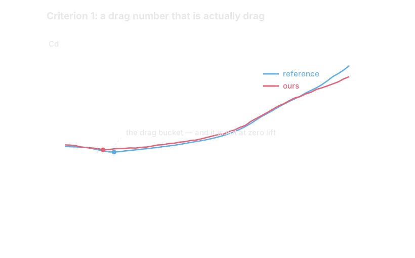
This passes. All thirty test cases are inside the ±15% bar, and — the part I like most — the drag bucket comes out right. Cambered sections have a minimum-drag angle that is not zero lift but somewhere near their design lift, because that is where the pressure distribution is gentlest on both surfaces at once. That is emergent here; nothing in the code knows about buckets.
It also gets the Reynolds trend right for the right reason. Drop a NACA 0012 from Re 10⁶ to 5×10⁵ and our drag goes 0.0059 to 0.0064, against a reference 0.0054 to 0.0062, because transition slides aft from 0.67 to 0.80 of chord and the cheap laminar run gets longer.
Go one step further down, to Re 2×10⁵, and it falls apart: we read 0.0067 against 0.0102. That one is worth staring at, because our transition point there is 0.97 against XFOIL’s 0.90 — barely different. The missing drag is not in the wrong place, it is a thing we do not model at all. Down there the laminar layer separates before it ever transitions, sits off the surface for a few percent of chord, goes turbulent in mid-air and comes back down. That is a laminar separation bubble, and it is expensive. My solver notices it happening and prints a warning. That is the whole of its bubble model.
The circular argument
Now the awkward part. The boundary layer needs to be told the speed at the edge of the layer, which comes from the frictionless solve. And the frictionless solve needs to be told the shape of the body, which — because of δ* — depends on the boundary layer.
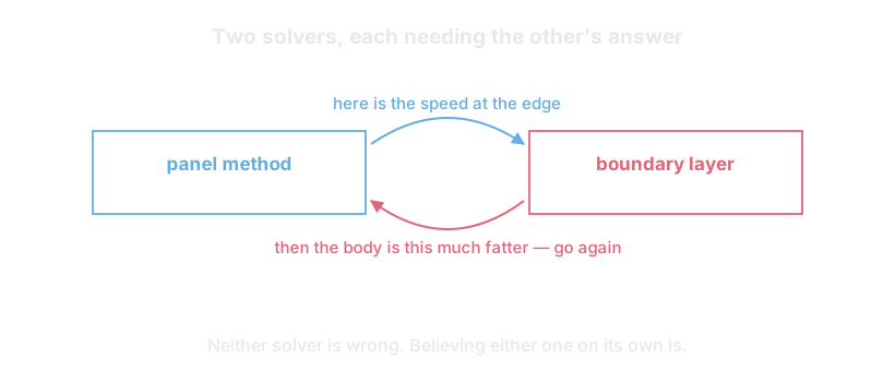
So you guess, and iterate. Solve the clean shape, march the layer, thicken the shape by δ* along the surface normals, re-panel it, solve again. It converges in 4 to 22 passes and the whole thing still runs in a few milliseconds, because the expensive part — factorising the influence matrix — is a couple of hundred rows.
Two refinements to that loop earned their place. It is a fixed-point iteration, so it responds well to standard acceleration — first Aitken’s method, then Anderson mixing, which keeps the last four residuals and solves a small least-squares problem for the next step. Neither changes the answer, only the path to it; Anderson took the matrix from 29 converged cases to 30.
That sounds like housekeeping and had a consequence I did not expect. The single case Anderson newly converged had been reporting a lift error of +0.038 from a final iterate the solver itself flagged as untrustworthy. Converged properly, it reads +0.056 — outside the tolerance. Every case in the failing set did the same thing: the harder they converge, the further they move from the reference. Better numerics did not create the error, it exposed it. That is a good feeling and a bad result.
The shape the air actually sees
Here is what the coupling is doing, physically. At any real angle of attack the boundary layer on top of the section is much thicker than the one underneath, because the top is the surface being asked to climb the pressure hill. So the fattened body is not fattened symmetrically — it is fattened mostly on top, mostly at the back.
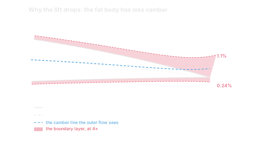
Which bends the effective camber line tail-up. Less camber means less lift, so the viscous answer sits below the frictionless one. That is viscous decambering, and it is the entire lift correction.
It is also, on this section, about half the size it ought to be: we take 0.038 off the frictionless Cl at 4° where the reference implies 0.079. The mechanism is right and the magnitude is short, which is criterion 2’s failure and most of the second half of this post.
The feedback is one line, and the @min in it is the one bit of dishonesty in the whole march:
const d = @min(surface.bl.h[k], DISPLACEMENT_H_CAP) * surface.bl.theta[k];
δ* is H times θ, and H is capped at 3.0 on the way out. Direct iteration of this kind has a genuine singularity at separation — push a boundary layer to zero wall shear in this formulation and the equations stop having a solution at all — so the cap keeps the loop bounded near the edge of trouble. Remember it; it comes back at the end, and not in the way I expected.
The bug that made the wing better at flying
The first version of this had the lift correction backwards. Viscous Cl came out above inviscid Cl, which is roughly like reporting that a rough wing works better than a smooth one.
The cause is a lovely one. The displaced body has to close: the trailing edge is a single sharp point, and if the top surface moves out by 1.1% and the bottom by 0.24%, the body has a hole in it. My fix was to taper δ* smoothly to zero over the last few percent of chord, so both surfaces came back to the original point.
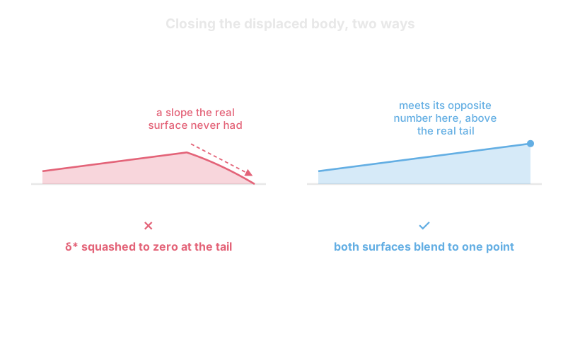
What that builds is a bulge at 95% of chord with a ramp behind it — which, to the outer flow, is a trailing-edge flap deflected downward by a degree or so. Aft camber is disproportionately good at making lift. So the taper made lift, and the taper was where the sign went wrong.
The way I found it was a parameter sweep, and the shape of the result is the tell. Shortening the ramp made it worse, monotonically: +0.034, +0.058, +0.083, +0.125, against a correct answer of −0.055. A thickness effect from a layer this thin would be an order of magnitude smaller than any of those, and it would not care how quickly the ramp closed. A flap would care very much.
The fix is that both surfaces now blend toward a single displaced trailing-edge point, the mean of what the two sides ask for. The body closes, no ramp, and — because the point is the mean — the camber part of the displacement survives while only the thickness part is discarded. Cl went from 3 cases in tolerance to 27.
A test written before the code
Before any of this existed I wrote down what it would have to reproduce, and committed the reference data. Nine published XFOIL polars for three sections at three Reynolds numbers, plus wind-tunnel anchors from Abbott and von Doenhoff and from the NPL, and five criteria with numbers attached. The rule in the project is that the implementation reproduces the data, never the reverse.
I recommend this to anyone building something like this. It is very easy to ship a plausible-looking aerodynamics tool that is quietly nonsense, and if you write the bar afterwards you will write it where you happen to be standing.
Here is where the solver stands today:
| criterion | result | |
|---|---|---|
| 1 | Cd within 15% | 30/30 |
| 2 | Cl within ±0.05 | 25/30 |
| 3 | drag bucket near design lift | 2/2 |
| 4 | stall onset, and Cl must flatten | 0/6 |
| 5 | transition within ±0.15 chord | 30/30 |
| convergence | 30/30 |
Overall: fail. Everything stays on the spike branch, nothing goes near the API, and every result the CLI produces carries a warning saying so.
The lift curve that never gives up
Criterion 4 is the interesting failure, and it is total: zero out of six.
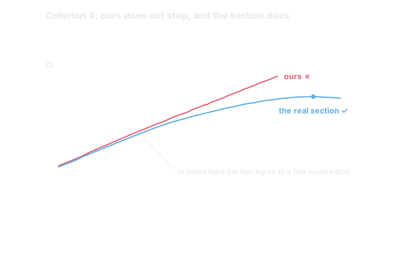
Real sections stop. Ours does not. Push the angle up and lift keeps rising, slightly below the frictionless line and just as straight — at 14° we report Cl 2.02 where the section really makes about 1.63 and is close to done.
What makes this worth writing about is that the boundary layer knows. On all six polars, the angle at which the solver’s own upper-surface separation crosses 90% of chord lands within 3° of the reference stall angle — worst miss 1.5° — and the lift slope below that matches the tunnel value of about 0.11 per degree. The layer sees the flow come apart at very nearly the right angle. The lift curve never hears about it.
That is a coupling failure, not a physics failure, and it has two halves.
The first is that cap on H. For two documents and about a week I believed that constant was what clamped the feedback. When I finally measured it, it is over-run at the trailing edge on only a handful of angles and never above 11°. What actually binds is elsewhere: once the march declares separation it holds the shape factor at that station’s value all the way to the tail, which pins H at the trailing edge to between 2.40 and 2.61 across a sweep to 18 or 20°, while the reference solution’s climbs to somewhere between 7 and 13. The mechanism I had written down was right. The constant I had blamed for it was not, and nothing but a measurement was ever going to tell me.
The second is that a closed body has no wake. The real circulation deficit at high loading is set partly by what the wake does behind the trailing edge, and there is no wake in this formulation — the body closes at a point and the story ends there. I spent a while trying to smuggle the effect in: probe the flow direction a few percent behind the tail, and deflect the displaced trailing edge to point along it. The mechanism is real, and it is the only intervention in the whole investigation that fixed the aft-loaded cases with the right sign and the right case-by-case variation, with no tuned constant anywhere.
It also never beat the baseline. Four different ways of deciding which part of that flow direction to subtract scored 23, 18, 24 and 22 cases against the baseline’s 26. The conclusion is not that the fourth one needed more work — it is that a probe five percent behind a closed body sits in the rear stagnation region, where the flow direction is dominated by the fact that the body is closed. There is no universal signature there to subtract, so no choice of datum can rescue it.
The tests are wrong too
Two of my own criteria do not measure what I told them to, and both are worth admitting.
Criterion 4 grades the angle at which the lift slope halves against the angle of maximum lift. Those are different quantities — on the reference data the slope break comes 1.5 to 5.5 degrees before the peak, which is outside my own ±3° tolerance on four of the six series. Run through this exact test, XFOIL scores 2 out of 6. That does not rescue me: we report no slope break at all in a sweep reaching 18° where the reference has one at 10 to 14. But a criterion that fails the reference implementation is measuring the wrong thing, and a future revision should grade a break angle against a break angle.
Criterion 5 has the opposite problem: it is too generous. Within ±0.15 of chord passes 30 out of 30 and always would have — it was written to catch a transition model that was absent or inverted, not to measure one. Against XFOIL run on my own geometry, my transition locations sit a near-uniform 0.037 of chord too far forward, on 50 of 58 surface-sides, 46 of them in the same direction. A systematic bias that consistent is a bug with a cause, and criterion 5 cannot see it at all. It came from integrating the amplification against the wrong variable; fixing that took the over-amplification from 25% to 1.9%, and criterion 5 did not move, because it never could.
The thing that looked like physics and wasn’t
One more, because it is the most instructive mistake in the whole exercise.
Early on, drag was 20 to 40% high and transition was consistently early. The cause looked obvious: on cambered sections at low Reynolds number the laminar layer separates, and I was treating that as an instant trip to turbulent — a crude bubble model. Removing that trip took criterion 1 from 15 cases to 28 and criterion 5 from 27 to 30, the largest single improvement in the project.
The obvious write-up is “we now model short bubbles better”. That write-up is wrong, and the measurement says so: with the trip removed, no case in the matrix laminar-separates at convergence at all. The trip had been firing during the first two or three coupling iterations, where the edge velocity is still the frictionless field with its steeper pressure gradient — and the code froze the transition location after three free iterations, so a transient from an early guess was being locked in and carried to the answer.
I had not fixed a bubble model. I had removed a mechanism that was capturing a wrong intermediate result. Freezing anything on an iteration count rather than a convergence measure is still in there, still not biting on this test matrix, and still exactly the shape of thing that will bite on a section I have not tried.
Next
The two open criteria have the same owner, which is why nothing has graduated: a viscous polar with untrustworthy lift is not a usable product, and there is no coherent subset to ship.
The fix is to stop iterating between two solvers and solve them as one system — every boundary-layer unknown, every edge velocity, and an explicit wake, in a single Newton solve of about seven hundred variables. That removes the singularity at separation, because the coupled system is well-posed where the direct march is not, and it gives the wake somewhere to exist. It is built. It converges on 23 of the 30 gate cases, it lands the aft-loaded lift cases the direct path misses back inside tolerance, and it has a habit of converging beautifully onto solutions that are not physical, which is its own long story.
That is the next post, and it has better failures than this one.
Everything here is measured rather than remembered — every number in this post came out of the solver or the committed reference data while I was writing it. If any of it is wrong, I would like to know.